The General Inquirer in the time of LLMs: a BERTopic tutorial

The General Inquirer, published in 1966, was the first algorithm attempting to recognise recurrent patterns in text data.

Introduction

What are the main issues addressed in a set of documents? Are those documents similar or discussing different matters? What is the most important topic? Delineating the main themes in a collection of documents is a common task in social sciences, particularly when exploring a new corpus. Although topics can, in principle, be identified manually, doing so becomes impossible when dealing with large corpora. For this reason, social scientists have long relied on topic modelling techniques to quickly extract the main themes present in their corpus (Asmussen & Møller, 2019), whether for exploratory purposes or to assign a label to individual document to conduct further analysis (DiMaggio et al., 2013).

Topic modelling is a natural language processing task that extracts latent topics structuring a corpus
For instance, Jockers & Mimno (2013) extracted broad themes in the English literature from the 19th century.
Several algorithms can perform this – for many years, LDA was the method de choix, now challenged by embedding-based approaches like BERTopic.

Natural language processing (NLP) is a subfield of computer science that analyses textual data. Main NLP tasks are text generation (like chatGPT), text classification, or topic modelling.

Figure 1: Topic Modelling in-out sketch

Until recently, topic modelling techniques — and natural language processing (NLP) in general — heavily relied on word counts, especially bag-of-words approaches. Amongst other limits, those approaches did not take into account the context in which a word is used — the order of the words in a sentence does not matter to those models, thus failing to grasp the complexity of the human language.

To tackle this limit, researchers developed approaches that generate richer and denser representations based on deep learning models. Those models take the text as an entry and generate a vector representation called embeddings. BERTopic is a topic model package written in Python that leverages embeddings generated by pre-trained transformer models¹ to delineate coherent topics based on the semantic similarity of texts.

Since its inception in 2022, BERTopic has proven its relevance in various studies. For instance, Bizel-Bizellot et al. (2024) used it to analyse survey-free-text answers and identified the main circumstances of infection with COVID-19. In a different field, Törnberg & Törnberg (2025) analysed images and texts to highlight trends regarding misinformation on climate.

BERTopic is a useful tool, but mastering it may feel demanding. In this tutorial, we focus on the general philosophy and how to use BERTopic for a social science project. We will demonstrate how to start with a text corpus and create a topic model that makes sense. We will create a topic model of the PhD theses defended between 2010 and 2022 in France to describe what keeps French PhD students busy.

By the end of this tutorial, you should be able to:

• Get an idea of what you can do with topic modelling in social science
• Set up a topic model on your data and make sense of the results
• Understand each step of the BERTopic pipeline and customise it

We conclude this tutorial with a discussion on good practices for reproducibility.

Python, Machine Learning and NLP prerequisites

We don’t assume that you have any knowledge about NLP and try our best to explain every step in an agnostic manner. We also provide numerous references for those who want to dig deeper.

Nevertheless, you will need to have some notions of Python. If you need to refresh your Python skills, you can use Lino Galiana’s courses. We assume that:

• you have a working environment and can install packages
• you know the basic syntax of Python (functions, variables, if-statements, for loops) and you’re comfortable enough with Pandas to load your documents and proceed to simple manipulations such as creating, dropping and renaming columns and rows.

In this tutorial, we use Python 3.12, and you can install the packages we will need with :

pip install -U bertopic pandas scikit-learn datasets plotly kaleido stopwordsiso nbformat ipykernel

Note

We provide a detailed “requirements” file that should work for Linux and MacOS.

bertopic==0.17.3
datasets==4.3.0
hdbscan==0.8.40
numpy==2.3.5
pandas==2.3.3
plotly==6.3.1
scikit_learn==1.8.0
stopwordsiso==0.6.1
transformers==4.52.4
umap_learn==0.5.7

Material

The tutorial comes with some material uploaded on Zenodo :

• A Jupyter notebook with code to execute
• The original dataset (which can be downloaded here)
• A clean dataset with the cleaning code

The notebook is available on Github.

Understanding BERTopic

The BERTopic pipeline

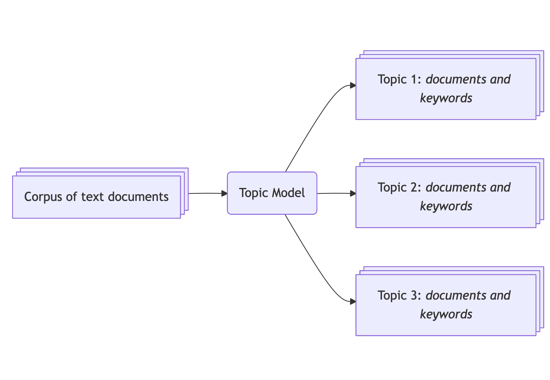
The BERTopic pipeline takes a list of text documents and returns meaningful topics as well as a mapping from the text documents to the said topics. The goal is to be able to gather documents that are semantically close into clusters, and then describe these topics for further interpretation. Once you have a set of topics, you can come back to the corpus to describe its composition.

Here is a basic usage of BERTopic which uses the main methods :

from bertopic import BERTopic

# Load your documents
documents = [
    "My cat is the cutest.",
    "Offer your cat premium food.",
    "The Empire State Building is 1,250 feet tall.",
]

# Create a BERTopic object
topic_model = BERTopic()

# Fit your model to your documents
topic_model.fit(documents)

# Predict the topics and probabilities
topic, probabilities = topic_model.transform(documents)

# Or do it all at once
topic, probabilities = topic_model.fit_transform(documents)

Note

The methods fit, transform, and fit_transform belong to a common syntax in machine learning systematized by Scikit-learn, one of the first and most complete machine learning library in Python. A vanilla model is fitted on the data (parameters are tweaked), and then the model is used to make predictions on new data.

The transformation produces two outputs.

• The topic variable is a list containing integers: for each document, the integer represents the topic/group it belongs to. In our case, topic = [0, 0, 1] as the first 2 documents mention cats, whereas the last document is about the Empire State Building.
• The probabilities variable is a list of floats: for each document, the float represents how close it is to the topic.

We can then retrieve topic information that will return keywords that best represent our corpus:

topic_info = topic_model.get_topic_info()

The topic_info variable is a table like this :

Table 1: Topic information for a simplified corpus

Topic	Count	Name	Representation	Representative_Docs
0	2	0_cat	“cat”	“My cat is the cutest”
1	1	1_building	“building”	“The Empire State Building is 1,250 feet tall”

The Topic column lists the topic IDs, the Count column lists the number of element there are in each topic, the Name column is a summary of topic ID and keywords — listed in the Representation column, and finally the Representative_Docs lists example of documents that are representative of the topic.

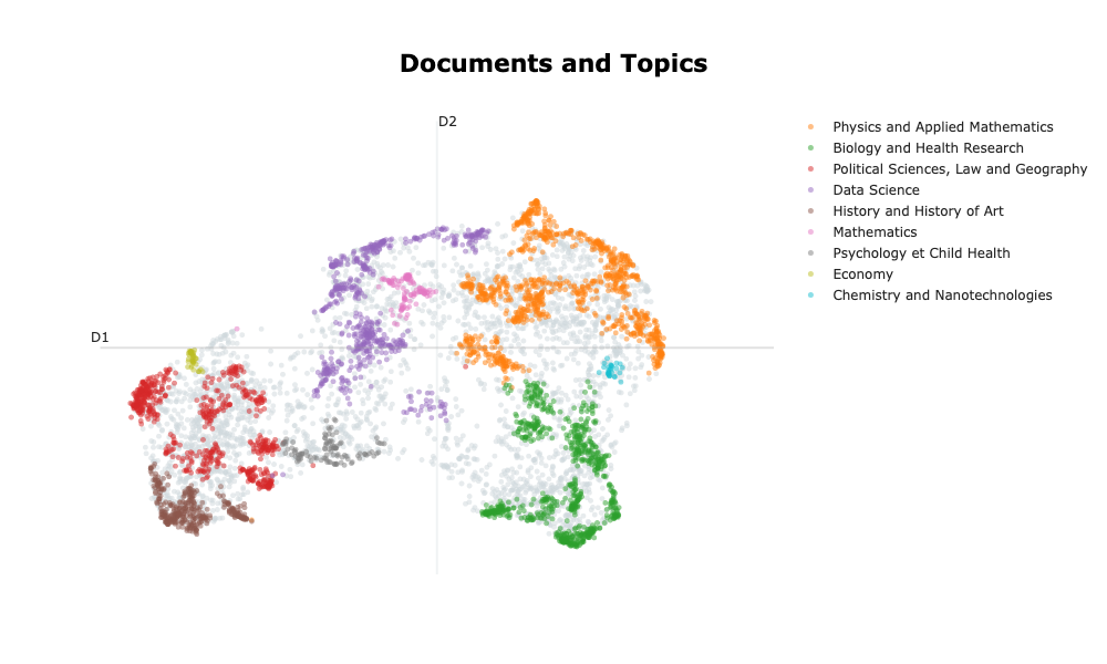
In reality, this example would not run because there are not enough documents! Let’s have a look at what one can expect from BERTopic, working with a real dataset: the abstracts of all the theses defended in France since 2010. After carefully setting the parameters and verifying the topic model’s quality, we obtain the following results:

Table 2: Topic information of the French theses after tuning the topic model

Topic	Count	Name	Representation
0	1601	Physics and Applied Mathematics	model study material property method phase surface field process thesis
1	1275	Biology and Health Research	cell gene protein study expression role species response involve mouse
2	1156	Political Sciences, Law and Geography	law legal study french language international teacher analysis public social
3	1030	Data Science	propose datum model method base approach network thesis application algorithm
4	631	History and History of Art	literary century study writing art time author history narrative period
5	202	Mathematics	graph prove study space class thesis chapter theorem random theory
6	328	Psychology et Child Health	study child patient infant adolescent disorder preterm social age intervention
7	105	Economy	monetary bank policy economic chapter financial country banking credit growth
8	172	Chemistry and Nanotechnologies	emulsion hydrogel microgels casein surface collagen property droplet quercetin gel

Figure 2: 2D plot of the French theses after tuning the topic model — grey dots are classified as “noise”; these elements can be reassigned a category as we will describe later.

Breaking down the process

Under the hood, BERTopic does three main steps:

• Generate a mathematical representation of each document that captures the semantic properties — the embeddings.
• Based on the embeddings, identify groups of documents that are semantically close (this action is called clustering). The hope is that these groups represent latent topics of the corpus.
• For each identified topic/group, retrieve keywords that best describe the specificity of each topic.

How to generate the embeddings?

To generate the embeddings, we use encoder models. Encoder models are a type of pre-trained transformer model² whose job is to encapsulate the semantics of textual data. A good example of an encoder is the BERT model and all its successors, like RoBERTa or DeBERTa. By default, BERTopic uses a package called sentence-bert, or SBERT, for generating embeddings.
Encoder models can take in a limited number of tokens (parts of words); this is called the context window size. For smaller models, the context window size is about 500 tokens (200 words on average), like for BERT, and larger models like ModernBERT have a context window size of 8,000 tokens.

Learn more about embedding techniques

• BERTopic documentation on embeddings
• “The illustrated Transformer” by Jay Alammar
• A visual explanation of general concepts behind LLMs by 3Blue1Brown

The embeddings — ie the generated vectors, contain hundreds of dimensions (for instance, the dimension of BERT’s embeddings is 512). Clustering algorithms work poorly with this many dimensions so we need to reduce the dimensionality of the embedding space (typically between 2 and 10). To reduce the dimensionality, the BERTopic pipeline uses the UMAP algorithm for its ability to grasp local and global structures (McInnes et al., 2018)³. This means that, despite moving from several hundred dimensions to only a couple, documents that are close together will stay close and distant ones will stay further apart. This is a critical step as we are heavily changing the structure of the data.

Learn more about dimensionality reduction and UMAP

• “What is dimensionality reduction?” by Eda Kavlakoglu (IBM)
• UMAP documentation
• Youtube videos to understand the main ideas (StatQuest) and the mathematical details (StatQuest).
• To explore the impact of the UMAP parameters.

How to generate clusters

The goal for the clustering algorithm is to create groups of documents that are semantically close. We are not certain that the output clusters will be “real” topics, ie. meaningful. In fact, as it often happens with these methods, some clusters make no sense, some should be merged, other separated.
But our intention is to tune the BERTopic pipeline in order for the clusters to be representatives of topics that are latent in our corpus.

Different algorithms can be used for clustering. HDBSCAN was chosen for its ability to detect clusters based on their density, hence it is able to detect clusters of various shapes and densities. HDBSCAN also allows for documents to be labelled as noise to primarily focus on dense and coherent groups.

Learn more about clustering techniques and HDBSCAN

• Clustering by Scikit-Learn
• Presentation of HDBSCAN by John Healy - PyData NYC 2018
• The HDBSCAN documentation
• The Scikit-Learn documentation of HDBSCAN

How to describe topics / retrieve keywords

Once we have created groups of documents, we need to create a meaningful representation of these topics. The general idea in BERTopic is to identify keywords that best describe the specificity of each topic.

To achieve that, it needs to come back to all the texts in the cluster and sparse them at the word level⁴. It uses word-count-based techniques that will count the number of occurrences of each word⁵. There are different strategies to make this word-count-based representation better. For instance, we can choose to remove stop-words — words that do not carry much semantic information (ex: “the”, “I”, “is”, “but”, … ). Other solutions include lemmatisation of words to consider “cats” and “cat” as one word.

The idea is to create a word x document matrix. The most basic strategy is to use the CountVectorizer object from scikit-learn which will create a word x document matrix.

Example

Given the two following documents:

• “My cat is the cutest.”,
• “Offer your cat premium food.”,

The word x document matrix would be:

	doc 1	doc 2
cat	1	1
cutest	1	0
offer	0	1
premium	0	1
food	0	1

In contemporary text analysis, the word x document matrix is seldom used. A usual transformation is called TF-IDF, as it highlights words that matter most. In practice, it gives more importance to words that appear often in a document and decreases the score of words that appear in many documents. BERTopic uses an alternative option called c-TF-IDF. This transformation raises the score of words that appear often in documents of the same group and decreases the score of words appearing in other groups. With this transformation, we retrieve words that make a group unique!

Learn more about bag-of-words and TF-IDF

• “N-gram Language Models” Chapter 3 of Speech and Language Processing by D.Jurafsky and J.H.Martin
• Tutorial TF-IDF with Scikit-Learn

Conclusion

To sum it up we have:

• First, generate embeddings that encapsulate semantic information with SBERT and reduce the dimensionality of vectors to a manageable number of dimensions with UMAP.
• Then create groups of semantically proximate documents with HDBSCAN. Each group can represent latent topics in our corpus.
• Create meaningful representations of each group by counting words in the documents with CountVectorizer and outline the most representative words with c-TF-IDF.

Figure 3: The 6 steps of BERTopic source

Note

The Optional Fine-tuning step is not covered in this tutorial. This step proposes to use generative LLMs to describe the topics.

BERTopic pipeline: the essentials

Preprocess your data

As mentioned before, we will use the dataset listing all dissertations defended in France since 1985. The original dataset can be downloaded on data.gouv.fr. To avoid excessive pre-processing, we curated⁶ the dataset and uploaded it (with the code) on Zenodo.

It is crucial to stress that the preprocessing step is the most important step. Although we can tune the topic model towards meaningful clusters and representations, your corpus is your input and no model will generate good results out of poor inputs. We list a number of questions you need to consider and justify for your topic model to be relevant:

Is my corpus homogeneous enough?

It could be tempting to shove millions of different documents from different sources into a topic model and see what comes out. However, to make sure that the groups will represent topics, one must be sure that your documents are similar in formality, tone, length, density of information etc… If your corpus is too heterogeneous, the topic model can highlight these differences and you will lose sight of meaningful latent topics⁷.

In our case, as we analyse dissertation abstracts which are quite standardised, the corpus should be homogenous enough for the topic model to pick up topics and not other semantic dimensions. It is worth noting that using the abstracts as a proxy to analyse a corpus of papers is common practice (Ma et al., 2025; Ollion et al., 2025)

Are my documents in the right language?

Most of the time, language models are trained in a single language. Some models are called multi-lingual and accept texts in more than one language. However, in our experience, working with documents in different languages generates poor topics as the language shift holds for the most salient difference and each language is clustered by itself. We recommend translating your documents in a single language beforehand.

In our case, the data curation led us to extract dissertations where both the English and the French abstracts were provided and we will work with abstracts in each language separately.

How long are my documents?

One needs to precisely define their task before diving into topic modelling. What are you trying to analyse? Will this information be available at the sentence level? paragraph level? the document level?

In our case, the topic of the dissertations will be described throughout the abstract, hence the abstract must be taken as a whole and not subdivided at the sentence level.

Also, as introduced before, each embedding model has a context window, meaning that long documents will be truncated. One must make sure that the length of the documents in their corpus is smaller than the model’s context window. If the context window is too small consider changing embedding model. Careful though, larger context window means longer computation time and greater computation resources required to run the model.

We will confirm the length of our documents before using the embedding model.

Open your data

Let’s load the dataset:

import pandas as pd
df_raw = pd.read_csv("./data/theses-soutenues-curated.csv")

The dataset contains the following columns :

• CI: Custom index, values are CI-XXXX, with XXXX ranging from 0 to 164,378
• year: the year of the defence, values are integers ranging from 2010 to 2022
• oai_set_specs: the oai code, each code looks like ddc:XXX, for instance ddc:300 refers to Sciences sociales, sociologie, anthropologie.
• resumes.en and resumes.fr: the abstract of the PhD dissertation, respectively in English and French. We are sure that every row contains a valid abstract in the right language thanks to the data curation.
• titres.en and titres.fr: the titles of the PhD dissertation, respectively in English and French. Only 5% of the rows do not have a valid title (French or English). The language of the titles has not been checked because it will only be used to check the qualitative validity of topic model.
• topics.en and topics.fr: the aggregated topics provided by the author. Only 5% of the rows do not have valid topics (French or English). The language of the topics has not been checked because they will only be used to check the qualitative validity of topic model.

Let’s take some time to check if our documents fit inside the context window. To retrieve the context window size, you can check the HuggingFace page of the model or load the configuration file that contains this information as such:

from transformers import AutoConfig 
config = AutoConfig.from_pretrained(model_name, trust_remote_code = True)
print(f"Context window size of the model {model_name}: {config.max_position_embeddings}")

Let’s look at two models, sentence-transformers/all-MiniLM-L6-v2 (default embedding model in the BERTopic pipeline) and Alibaba-NLP/gte-multilingual-base.

>>> Context window size of the model sentence-transformers/all-MiniLM-L6-v2: 512
>>> Context window size of the model Alibaba-NLP/gte-multilingual-base: 8192

And now let’s look at the length of our documents:

df_raw["resumes.en.len"] = df_raw["resumes.en"].apply(len)
df_raw["resumes.fr.len"] = df_raw["resumes.fr"].apply(len)
df_raw.loc[:,["resumes.en.len", "resumes.fr.len"]].describe()

Descriptive statistics of the length of the abstracts in English and in French

	resumes.en	resumes.fr
min	1	6
25%	1324	1508
50%	1617	1702
75%	2080	2362
max	12010	12207
mean	1777	1984
std	735	802

With these statistics, we see that we can rule out using sentence-transformers/all-MiniLM-L6-v2 because it’s context window is too narrow. By keeping abstracts between 1000 and 4000 characters (ie between 300 and 1300 tokens⁸) we can retain most of the dataset (89%) while maintaining a reasonable computation time.

import numpy as np 
valid_index = np.logical_and.reduce([
    df_raw["resumes.fr.len"] >= 1000,
    df_raw["resumes.fr.len"] <= 4000,
    df_raw["resumes.en.len"] >= 1000,
    df_raw["resumes.en.len"] <= 4000,
])

df = df_raw.loc[valid_index,:]

Even if it is more interesting to process the complete dataset, it can be computationally expensive. To limit computation time at least for the exploratory steps, we are going to work on a sample of documents. To maintain some representativeness, we stratify this sampling by the year of the defence⁹.

stratification_column = "year"
samples_per_stratum = 500
df_stratified = (
    df
    .groupby(stratification_column, as_index = False)
    .apply(lambda x : x.sample(n = samples_per_stratum), include_groups=True)
    .reset_index()
    .drop(["level_0", "level_1"], axis = 1)
)
# Save the preprocessed dataset
df_stratified.to_csv("./data/theses-soutenues-curated-stratified.csv", index=False)

The resulting stratified table contains 6500 rows.

Create a BERTopic object, fit and transform

To create a topic_model object we need to create a BERTopic object and define some parameters. For now, we will not change the default parameters of the clustering model (hdbscan_model) or the dimension reduction model (umap_model). We will however define the language of the corpus as well as the vectorizer model in order to remove all stopwords and retrieve meaningful topics. Then, one must use the fit method to fit the topic model to the corpus.

from bertopic import BERTopic
from sklearn.feature_extraction.text import CountVectorizer
from stopwordsiso import stopwords

language = "english" # or "french"
language_short = language[:2] # "en" or "fr"
embedding_model = "Alibaba-NLP/gte-multilingual-base"
docs = df_stratified[f"resumes.{language_short}"]

vectorizer_model = CountVectorizer(stop_words = list(stopwords(language_short)))

topic_model = BERTopic(
    language = language,
    embedding_model = embedding_model,
    vectorizer_model = vectorizer_model,
)
topic_model.fit(documents=docs)

This snippet of code takes a long time to run (>10 mins) as each element must be embedded first.

To avoid unnecessary computation time, we have embedded 6500 elements with several models for the French and English abstracts that you can download from Zenodo. The code changes as such:

from bertopic import BERTopic
from sklearn.feature_extraction.text import CountVectorizer
from stopwordsiso import stopwords
from datasets import load_from_disk

language = "english" # or "french"
language_short = language[:2] # "en" or "fr"

# Load the embeddings directly to avoid long computation time
ds = load_from_disk(f"./data/embeddings/gte-multilingual-base-{language_short}-SBERT")
docs = np.array(ds[f"resumes.{language_short}"]) # 6500 rows
embeddings = np.array(ds["embedding"])           # Shape : 6500 x 768

vectorizer_model = CountVectorizer(stop_words = list(stopwords(language_short)))

topic_model = BERTopic(
    language = language,
    vectorizer_model = vectorizer_model,
)
topic_model.fit(documents=docs, embeddings=embeddings)

Now to extract the topics, we need to call the transform method :

topics, probabilities = topic_model.transform(documents=docs, embeddings=embeddings)

And to explore the topics we can call the get_topics_info method that will return a table with the keywords, representative documents and the number of documents in each topic:

topic_info = topic_model.get_topic_info()
topic_info

Table 3: Topic information (truncated) of the French dissertations for a basic topic model

	Topic	Count	Representation
0	-1	2715	[‘study’, ‘thesis’, ‘model’, ‘based’, ‘analysis’, ‘data’, ‘process’, ‘approach’, ‘development’, ‘social’]
1	0	262	[‘literary’, ‘writing’, ‘art’, ‘contemporary’, ‘authors’, ‘poetry’, ‘narrative’, ‘history’, ‘texts’, ‘poetic’]
2	1	172	[‘mechanical’, ‘numerical’, ‘behavior’, ‘material’, ‘crack’, ‘model’, ‘materials’, ‘experimental’, ‘element’, ‘finite’]
3	2	172	[‘cells’, ‘cancer’, ‘tumor’, ‘cell’, ‘immune’, ‘expression’, ‘patients’, ‘melanoma’, ‘tumors’, ‘response’]
4	3	155	[‘flow’, ‘numerical’, ‘fluid’, ‘acoustic’, ‘flame’, ‘flows’, ‘model’, ‘simulations’, ‘method’, ‘experimental’]
…	…	…	…
102	101	10	[‘influenza’, ‘vaccination’, ‘meningitis’, ‘virus’, ‘infection’, ‘pedv’, ‘nmx’, ‘h5n1’, ‘serogroup’, ‘dbs’]
103	102	10	[‘ablation’, ‘atrial’, ‘intracranial’, ‘vein’, ‘cardiac’, ‘fibrillation’, ‘icp’, ‘phantoms’, ‘catheter’, ‘veins’]
104	103	10	[‘building’, ‘ventilation’, ‘thermal’, ‘heat’, ‘cooling’, ‘wall’, ‘air’, ‘buildings’, ‘comfort’, ‘heating’]
105	104	10	[‘humins’, ‘tannins’, ‘biobased’, ‘foams’, ‘composites’, ‘tannin’, ‘biocomposites’, ‘cab’, ‘materials’, ‘lignin’]

The “Representation” column provides the keywords for each topic. We can see that the keywords retrieved for the noise cluster are very generic: “study”, “thesis”, “model”, “analysis”, “approach” and do not convey any meaningful information other than the fact that all documents are academic documents.

For each topic, the model identifies apparently consistent keywords :

• ‘mechanical’, ‘numerical’, ‘model’, ‘finite’, ‘element’: this cluster may be grouping dissertations related to numerical simulation in mechanics using the finite element method.
• ‘cells’, ‘cancer’, ‘tumor’, ‘immune’, ‘patients’: this cluster may be grouping dissertations related to cancer and cures.
• ‘building’, ‘ventilation’, ‘heat’, ‘cooling’: this cluster may be grouping dissertations related to the thermodynamics of buildings.

This is not a proof that our model generated interesting results, for that we need to carry further investigation of each cluster. Still this is a first step towards assessing the quality of the topic model.

In this table we can see that almost half of the documents are classified as noise (topic -1). This is a normal behaviour of the clustering algorithm as it focuses on dense areas first. This way, the topic model creates representations that focus fewer documents to retrieve very specific keywords. The other 104 topics contain between 10 and 200 documents each, which correspond to 0.1% to 3% of the corpus.

It is worth noting that the more documents in a cluster, the lower the topic index is.

It is possible to re-assign clusters to documents clustered as noise with the reduce_outliers method, based on the documentation and the code, we recommend using the “embedding” strategy¹⁰:

topics_reduced = topic_model.reduce_outliers(
    documents = docs, 
    topics = topics, 
    probabilities = probabilities, 
    embeddings = embeddings,
    strategy="embeddings" 
)

Warning

The topic model is not altered and keywords are not re-generated.

Visualise your results

Visualising your topics is central in topic modelling as this is the most convenient way to explore your documents and your topic model. We are going to cover some of the most basic and helpful visualisations.

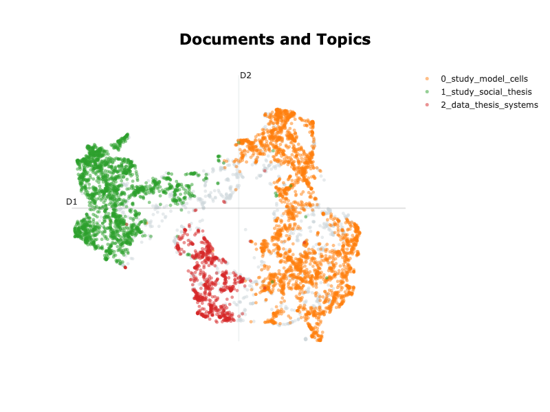
2D plot

The first thing we want to visualise is the space of the embeddings reduced to 2 dimensions. This is a good start to visualise the size of your clusters and if close clusters have similar topics.

(
    topic_model
    .visualize_documents(
        docs = docs,
        embeddings = embeddings,
        hide_annotations = True, # better readability
        topics = [0,1,2,3],      # Select topics to highlight
        # height = 300, # Adjust the height of the plot
        # width = 800 # Adjust the width of the plot 
    )
)

Figure 4: 2D plot of the French dissertations for a basic topic model¹¹

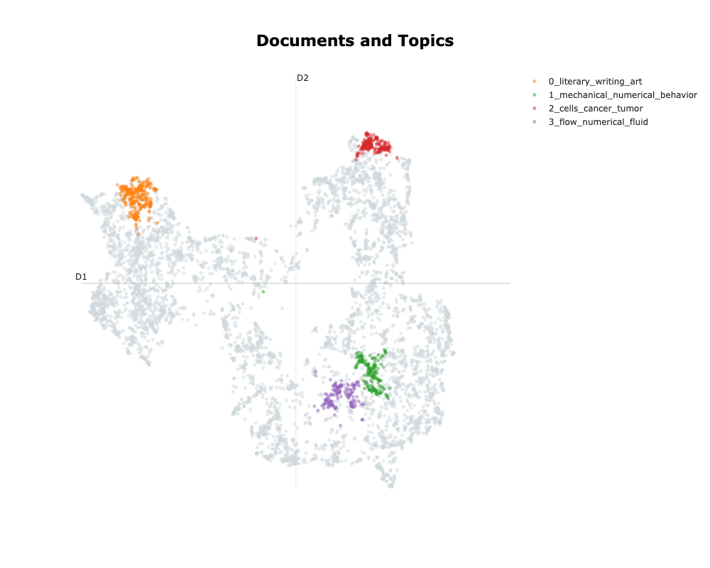
On this graph only displaying the 4 top topics, we can see that the cluster are large and dense. We can see that the “1_mechanical_numerical_behavior” and the “3_flow_numerical_fluid” are close, as expected whereas “0_literary_writing_art” and “2_cells_cancer_tumor” are further apart in separate directions.

Visualise top words per topic

The second helpful visualisation is to illustrate the top \(n\) words that represent each topic and how representative they are of a given topic. It is a good way to analyse the consistency of each topic and get a sense of the documents inside a cluster.

topic_model.visualize_barchart(
    n_words = 10, # Select the number of words to display per topic
    # topics = [0,1,2,3,4], # Select specific topics to display
    # top_n_topics = 6, # Select the first n topics to display
    # height = 300, # Adjust the height of the plot
    # width = 800 # Adjust the width of the plot 
)

Figure 5: Top \(n\) words per topic of the French dissertations for a basic topic model

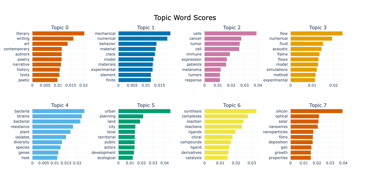
Take the topic n°5, we can see keywords like “urban”, “land”, “city”, “local”, “public” and “ecological”. These keywords make sense together and we can imagine dissertations discussing urban planning at different scales and under different constraints.

Hierarchical trees

A good way to visualise how topics interact with each other is to plot a dendogram. This plot is read from left to right, the sooner branches merge, the closer related topics are. We use the visualize_hierarchy method. The graph is very tall but we can easily focus on one subset of the tree at a time.

topic_model.visualize_hierarchy()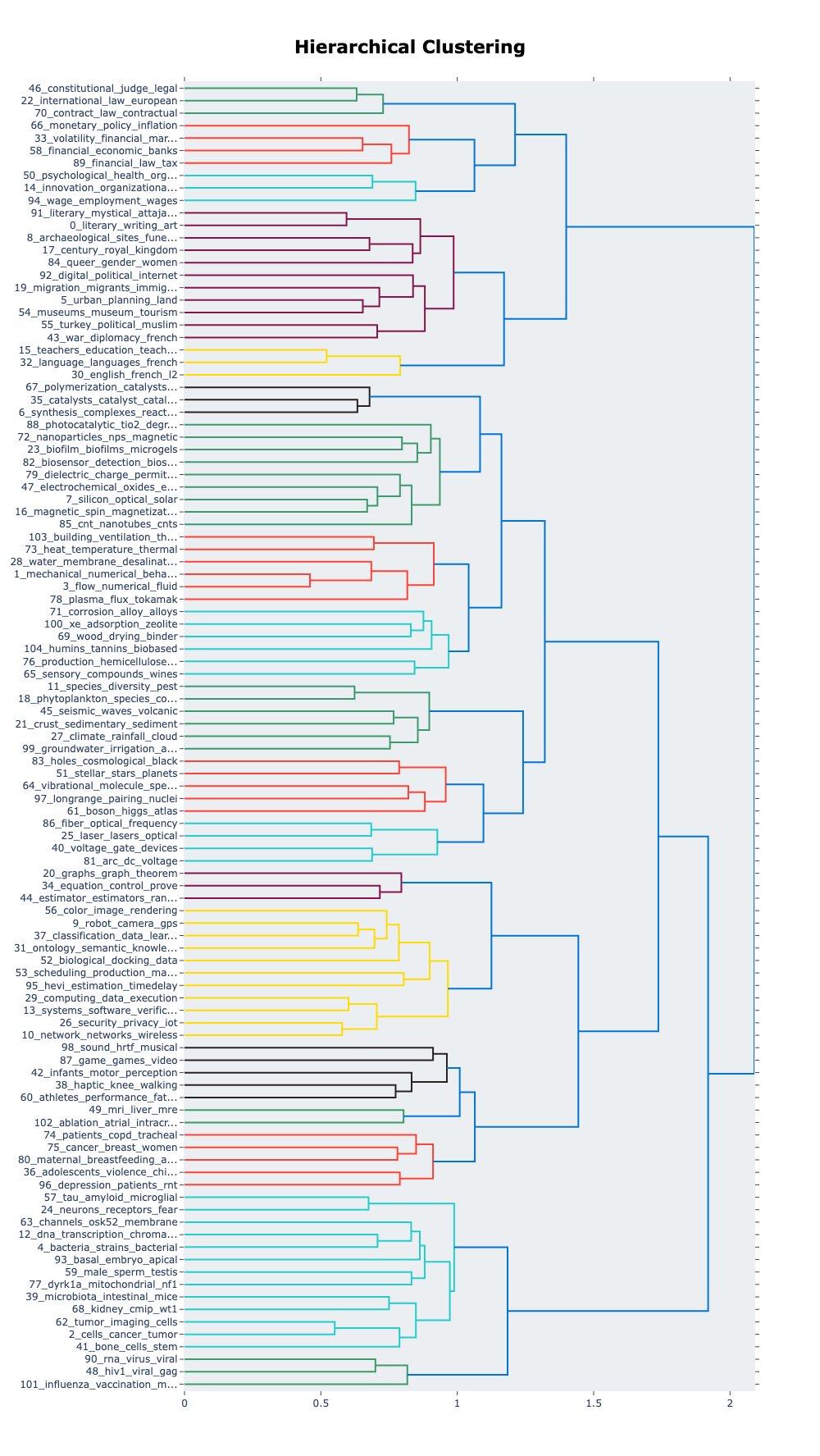

Figure 6: Hierarchical graph of the French dissertations for a basic topic model

At the very top of this graph, we can see the green branches related to laws and international law, very close to contract law. This is a sign that these three branches merge together and that we dont find legislation-related keywords anywhere else in the three.

BERTopic pipeline: advanced practices

Aggregate topics

Most of the time, the topic model will generate many groups, with some groups that you’d want to merge together.

To aggregate topics, the algorithm proposed is to use the topic embedding (the mean of the document’s embedding inside a cluster), compute the cosine similarity¹² matrix and use the agglomerative clustering algorithm described here to aggregate the topics. Once performed, all the documents are moved into a new group and keywords are re-generated.

With more than 100 topics, it is difficult to have a general idea of the main groups in the corpus. Looking back to the Figure 6¹³ we can identify seven large branches we could reduce our topic model to.

topic_model.reduce_topics(docs = docs, nr_topics=7 + 1) #Add one to account for the noise
#Retrieve the updated topics and probabilities
topics_reduced, probabilities_reduced = topic_model.topics_, topic_model.probabilities_

Then check the new representations like in the Section 3.3.

topic_info_reduced = topic_model.get_topic_info()
topic_info_reduced

Table 4: Topic information after aggregating topics

Count	Name	Representation
2715	-1_study_thesis_model_based	[‘study’, ‘thesis’, ‘model’, ‘based’, ‘analysis’, ‘data’, ‘approach’, ‘process’, ‘development’, ‘properties’]
1037	0_study_analysis_social_thesis	[‘study’, ‘analysis’, ‘social’, ‘thesis’, ‘french’, ‘political’, ‘century’, ‘approach’, ‘time’, ‘history’]
795	1_cells_cell_expression_role	[‘cells’, ‘cell’, ‘expression’, ‘role’, ‘species’, ‘study’, ‘patients’, ‘protein’, ‘cancer’, ‘involved’]
707	2_model_numerical_study_method	[‘model’, ‘numerical’, ‘study’, ‘method’, ‘experimental’, ‘thesis’, ‘flow’, ‘based’, ‘models’, ‘properties’]
634	3_data_thesis_systems_model	[‘data’, ‘thesis’, ‘systems’, ‘model’, ‘propose’, ‘based’, ‘approach’, ‘proposed’, ‘network’, ‘time’]
464	4_properties_magnetic_surface_synthesis	[‘properties’, ‘magnetic’, ‘surface’, ‘synthesis’, ‘materials’, ‘studied’, ‘study’, ‘temperature’, ‘nanoparticles’, ‘reaction’]
135	5_law_legal_international_rights	[‘law’, ‘legal’, ‘international’, ‘rights’, ‘european’, ‘monetary’, ‘financial’, ‘constitutional’, ‘policy’, ‘economic’]
13	6_detection_biosensor_biosensors_based	[‘detection’, ‘biosensor’, ‘biosensors’, ‘based’, ‘dna’, ‘sers’, ‘surface’, ‘splitaptamer’, ‘spr’, ‘sensor’]

Similarly to before, the noise topic contains very generic keywords. As for the rest, we can identify seven¹⁴ main latent topics :

• Social Sciences
• Medicine and Health
• Engineering Sciences, Experimentation and Simulation
• Data analysis and Mathematics
• Physics
• Law, Finance and Policies
• Biochemisty and sensors

The topics are very general and give us key insights about our corpus.

A detailed analysis can be useful to understand the structure of the corpus. For instance, the keywords for the second main topic are too general, but because we analysed our documents in details, we know that this topic is the result of merging “1_mechanical_numerical_behavior” and “3_flow_numerical_fluid”, allowing us to name this topic “Engineering Sciences, Experimentation and Simulation”.

After reducing outliers, here is the distribution of topics across all out documents :

Table 5: Repartition of the theses in the 7 aggregated topics

	Topic	Count	Proportion
Social Sciences	0	1749	27 %
Medicine and Health	1	1328	20 %
Engineering Sciences, Experimentation and Simulation	2	1106	17 %
Data analysis and Mathematics	3	1073	17 %
Physics	4	803	12 %
Law, Finance and Policies	5	410	6 %
Biochemisty and sensors	6	31	0 %

Finally, the 7th topic still seems very specific, even after reducing outliers, there are only 31 documents in this topic.

Note

You can merge topics by hand using the merge_topics method.

topics_to_merge = [1, 2, 3]
topic_model.merge_topics(docs, topics_to_merge)

Tune parameters

A diversity of parameters can be used to tune the topic model. In this section, we propose to tune the 3 most useful parameters outlined in the litterature: the embedding model, n_neighbors (UMAP) and n_components (HDBSCAN). A table can be found in the techy notes providing descriptions for other parameters.

1. Assess the quality of the text representations (parameter tuned: embedding model)

The primary factor to tune is the embedding model, because it drastically impacts the results of the topic model. To check if the embedding makes sense, you can plot the 2D map after dimension reduction with UMAP (n_components=2). Then, by exploring the map, you can assess if the embedding space created placed similar documents together or not.

At this point you can also try different values for n_neighbors and n_components. However, be aware that the influence of UMAP parameters on the final topic model is difficult to appreciate at first glance.

2. Tune the granularity of the topic model (parameters tuned: n_neighbors and min_cluster_size)

Once you’ve chosen an embedding model, you can change the n_neighbors and min_cluster_size. Both work jointly: the lower these parameters, the smaller the grain and the more specific the topics. It is worth noting that these parameters are dependant of the size of your corpus. For a corpus of 5,000 documents, n_neighbors=300 is a large value, but for 50,000 documents it might be a medium value.

To change these parameters, one must explicitly declare UMAP and HDBSCAN objects and pass them on to the BERTopic model:

from umap import UMAP
from hdbscan import HDBSCAN

# Load data and create the vectorizer model like before
language = "english" # or "french"
language_short = language[:2] # "en" or "fr"
ds = load_from_disk(f"./data/embeddings/gte-multilingual-base-{language_short}-SBERT")
docs = np.array(ds[f"resumes.{language_short}"]) # 6500 rows
embeddings = np.array(ds["embedding"])           # Shape : 6500 x 768
vectorizer_model = CountVectorizer(stop_words = list(stopwords(language_short)))

# create an HDBSCAN and UMAP models
hdbscan_model = HDBSCAN(
    min_cluster_size=50, 
    # Default parameters 
    prediction_data=True
)
umap_model = UMAP(
    n_neighbors = 50,
    # Default parameters
    metric = "cosine",
    n_components = 5,
    min_dist=0.0,
    low_memory = False 
)

# Then create the instance, fit the model and extract the topics and probabilities
topic_model = BERTopic(
    language = language,
    vectorizer_model = vectorizer_model,
    umap_model= umap_model,
    hdbscan_model=hdbscan_model
)
topics, probabilities = topic_model.fit_transform(
    documents=docs, 
    embeddings=embeddings
)

We obtain the following results:

Table 6: Topic information for a coarse grained topic model

Topic	Count	Representation
-1	837	[‘thesis’, ‘model’, ‘study’, ‘data’, ‘based’, ‘method’, ‘analysis’, ‘developed’, ‘approach’, ‘time’]
0	2917	[‘study’, ‘model’, ‘cells’, ‘properties’, ‘thesis’, ‘cell’, ‘studied’, ‘based’, ‘role’, ‘development’]
1	2011	[‘study’, ‘social’, ‘thesis’, ‘law’, ‘analysis’, ‘political’, ‘french’, ‘public’, ‘based’, ‘approach’]
2	735	[‘data’, ‘thesis’, ‘systems’, ‘propose’, ‘based’, ‘model’, ‘approach’, ‘proposed’, ‘network’, ‘methods’]

Figure 7: 2D map for a coarse grained topic model

Additional visualisations: cross-reference with additional tags

If you have additional tags for your dataset, such as categories or dates, you can easily display your topic analysis in regard of these dimensions.

In our case, we have OAI codes that account for the field each thesis is in. Hence we can compare the generated topics with the fields.

# some theses are in multiple fields, 
# the oai code is: 
# ddc:XXX||ddc:YYY
# for simplicity, we are going to keep the first field for each thesis
first_oai = [oai_code[:7] for oai_code in ds["oai_set_specs"]]

# Let's translate that to human language:
oai_names = {
    "ddc:300" : "Sciences sociales, sociologie, anthropologie",
    "ddc:340" : "Droit",
    "ddc:004" : "Informatique",
    "ddc:570" : "Sciences de la vie, biologie, biochimie",
    "ddc:540" : "Chimie, minéralogie, cristallographie",
    "ddc:620" : "Sciences de l'ingénieur",
    "ddc:550" : "Sciences de la terre",
    "ddc:530" : "Physique",
    "ddc:510" : "Mathématiques",
    "ddc:610" : "Médecine et santé"
}
def retrieve_name(oai_code):
    if oai_code in oai_names:
        return oai_names[oai_code]
    else : 
        return "Autre"

first_oai_names = [retrieve_name(oai_code) for oai_code in first_oai]

topics_per_class = topic_model.topics_per_class(docs, classes=first_oai_names)
topic_model.visualize_topics_per_class(
    topics_per_class,
    topics = [0, 1, 2, 3], # choose specifically which topics to display
    # top_n_topics = 10,   # choose to display the 10 largest topics
)

Figure 8: Topics distributed over the OAI tags of the French theses for a basic topic model

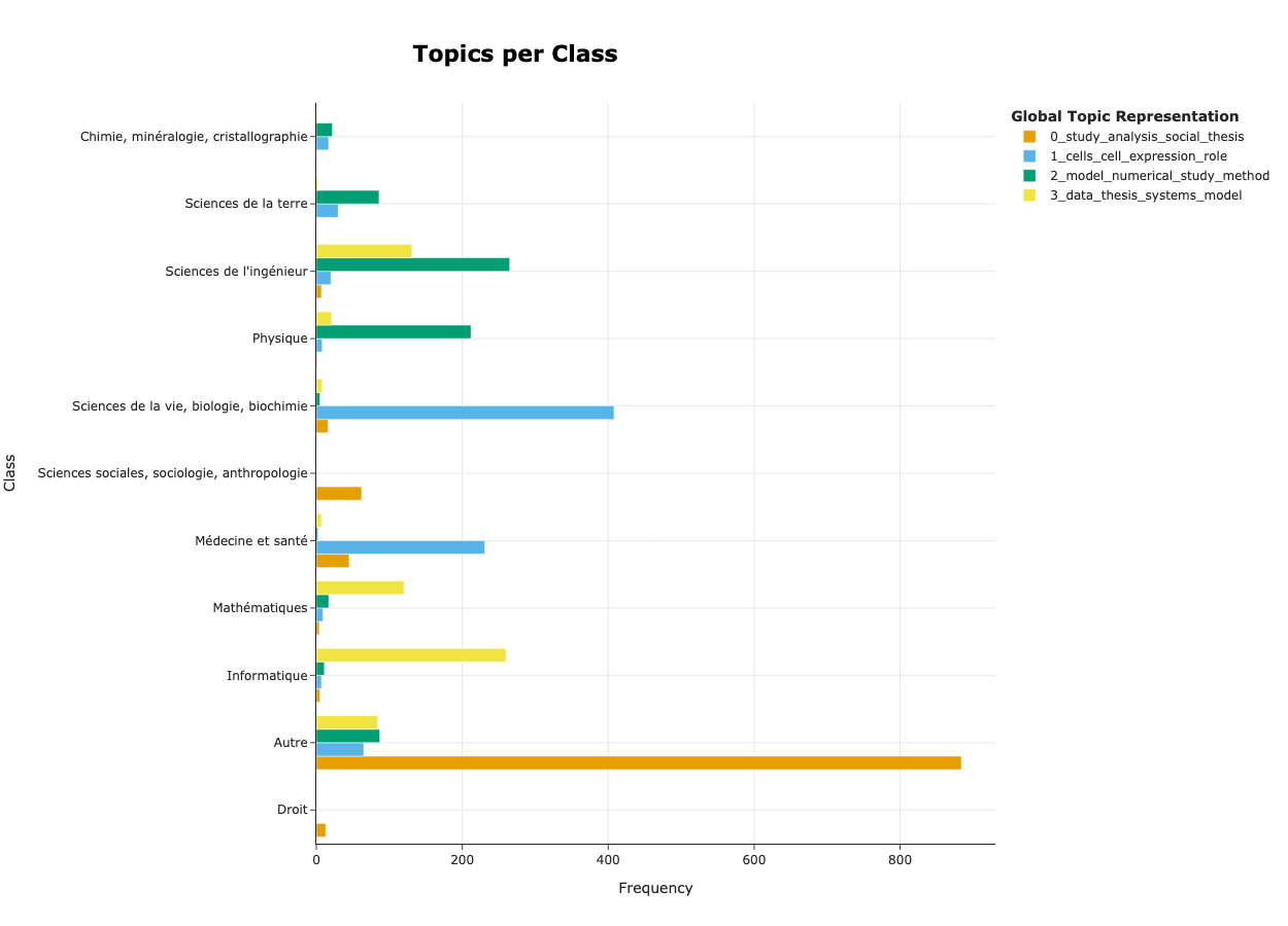
In this figure, we can start by checking that documents are associated to the right topic. For instance, it is coherent to see that documents of the topic ‘1_cells_cell_expression_role’ are found in theses in Health and Medicine as well as in Biology and Biochemistry and that documents of the topic ‘2_model_numerical_study_method’ are found in theses in Physics and Engineering science, .

If you want to visualise your topics on a temporal axis, you can use the the visualize_topics_over_time method.

year = [int(float(year_as_string)) for year_as_string in ds["year"]]
topics_over_time = topic_model.topics_over_time(docs = docs, timestamps=year)
topic_model.visualize_topics_over_time(topics_over_time, topics = [0,1,2,3])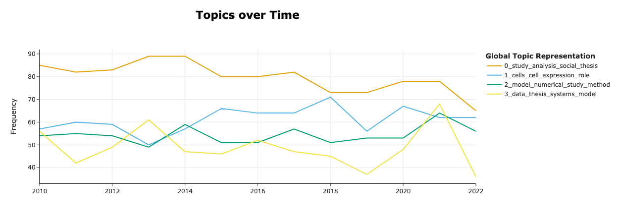

Figure 9: Number of theses over the years in each group of the French theses for a basic topic model

Evaluate your topic model

Topic model evaluation is an active domain of research that goes beyond the scope of this tutorial. We propose an overview of the methods that exist and how to quickly tell if your topic model can be used or needs to be refined.

In short: quantitative methods are impractical and one should focus more on the qualitative evaluation.

Qualitative evaluation

Throughout this tutorial, we have displayed many results and analysed them with the objective to answer the very question: is the topic model consistent? There is no one way around qualitatively evaluating your BERTopic, however the point is to offer some techniques we found useful and code snippets to quickly obtain key insights on your topic model performance.

Extensively use the visualisation tools

As presented in Section 3.4 and Section 4.3, there are many tools to visualise the results of your topic model that can help you assess the coherence of the topics through 2D representation, top n words, hierarchical and the tag distribution.

Explore the merging process

When merging topics at Section 4.1 we may want to monitor what’s going where. The following snippet prints out the topics that were merged into them:

for iRow_reduced, topic_id in enumerate(topic_info_reduced["Topic"]):
    print(topic_info_reduced.loc[iRow_reduced, "Name"].replace("_", " "))
    og_topics_merged_to_new_topic = list(set([
        int(og_topic) 
        for og_topic, new_topic in zip(topics, topics_reduced) 
        if new_topic == topic_id
    ]))
    for og_topic in og_topics_merged_to_new_topic:
        print(
            "\t - ",
            topic_info.loc[
                topic_info["Topic"] == og_topic,
                "Name"
            ]
            .item()
            .replace("_", " ")
        ) 
    print("---")

>>> ...
>>> 5 law legal international rights
>>>  -  66 monetary policy inflation exchange
>>>  -  70 contract law contractual subsidy
>>>  -  46 constitutional judge legal council
>>>  -  22 international law european rights
>>>  -  89 financial law tax transactions
>>>  -  58 financial economic banks growth
>>> ...

In this example we can confidently assess that the merge is coherent as it groups all law related topics into one.

Explore the reason why a given document was clustered in a specific group

The topics_per_class is a powerful method that retrieves top keywords found in specific documents that justify assigning it to a given cluster:

# Select a document
text_id = 3000
is_my_document = [i == text_id for i in range(len(docs))]
print(f"Doc n°{text_id}:\n{docs[text_id]}")

topics_per_class = topic_model.topics_per_class(docs, classes = is_my_document)
topics_per_class = topics_per_class.loc[topics_per_class["Class"], :].set_index("Topic")
# Retrieve the Topic Representation for comparison
topics_name = (topic_model.get_topic_info().set_index("Topic")["Name"])
topics_per_class.loc[:,"Topic Name"] = topics_name
print(topics_per_class.reset_index().to_markdown())

>>> Doc n°3000:
>>> The overall objective of this thesis is to exploit a ...

Topic	Words	Frequency	Class	Topic Name
3	social, annotations, multimedia, snapshot, proposed	1	True	3_data_thesis_systems_model

If you have additional tags, it’s even more powerful as you can check the keywords for a whole class:

OAI_REFS = pd.read_csv("./data/oai_codes.csv")
DS = ds
def get_docs_for_oai_code(oai_code : str):
    try: 
        oai_name = OAI_REFS.loc[OAI_REFS["code"] == oai_code, "name"].item()
    except Exception:
        print(f"oai code {oai_code} invalid\n\nException:\n{Exception}")
        return
    
    def return_name(codes):
        if oai_code in codes: 
            return oai_name
        else: 
            return "Autre"

    classes = [return_name(codes) for codes in ds["oai_set_specs"]]
    topics_per_class = topic_model.topics_per_class(docs, classes = classes)
    topics_per_class = topics_per_class.loc[topics_per_class["Class"] == oai_name, :].set_index("Topic")
    topics_name = (
        topic_model
        .get_topic_info()
        .set_index("Topic")
        ["Name"]
    )
    topics_per_class.loc[:,"Topic Name"] = topics_name
    return topics_per_class.loc[topics_per_class["Class"] == oai_name, :].reset_index()

get_docs_for_oai_code("ddc:300")

Topic	Words	Frequency	Class	Topic Name
-1	social, thesis, study, public, political	98	Sciences sociales, sociologie, anthropologie	-1_study_thesis_model_based
0	social, study, thesis, french, analysis	73	Sciences sociales, sociologie, anthropologie	0_study_analysis_social_thesis
3	markov, volatility, smc, stochastic, em	1	Sciences sociales, sociologie, anthropologie	3_data_thesis_systems_model

Quantitative evaluation

In this section we introduce different metrics that can be used to evaluate your topic model. However, we mainly included it to warn you of the complexity behind evaluating a topic model and that there is no one-size-fit-all solution.

Response to “How to evaluate the performance of the model?” by Maarten Grootendorst source

First, choosing the coherence score by itself can have a large influence on the difference in performance you will find between models. For example, NPMI and UCI may each lead to quite different values. Second, the coherence score only tells a part of the story. Perhaps your purpose is more classification than having the most coherent words or perhaps you want as diverse topics as possible. These use cases require vastly different evaluation metrics to be used.

There are two types of metrics that you could use:

• Cluster metrics — ie focus on the group-making. There exist a lot of metrics, but few are fit to our situation: unsupervised learning with density based algorithms. In our experience, optimising these metrics results in a sub-optimal solutions as illustrated bellow. Read more
• Topic representation metrics — ie focus on how relevant the keywords are. Although some metrics exist their utility is limited: good score does not necessarily align with what expert consider good topic models, and they are not good scores to optimise (Stammbach et al., 2023). Read more

Some good practices

Now that you have a good understanding of BERTopic, and you started to experiment with it, you may want more practical advices. Here, we list some tips to reduce computation time and facilitate reproducibility.

Save your instance locally

For reproducibility purposes, BERTopic lets you save the BERTopic object you created with the save¹⁵ method. Two parameters of importance:

• serialization (str): must be "safetensors", "pickle" or "pytorch". We recommend using "safetensors" or the "pytorch" format as they are broadly used in machine learning and recommended by the BERTopic documentation.
• save_ctfidf (bool) : wether to save the vectorizer configuration or not. This is the heaviest bit (see table below).

# ~ 500 KB
topic_model.save(
    path = "./bertopic-default",
    serialization = "safetensors",
    save_ctfidf = False
)

# ~ 6MB
topic_model.save(
    path = "./bertopic-default-with-ctfidf",
    serialization = "safetensors",
    save_ctfidf = True
)

To reload your instance you just need to use the load method:

topic_model = BERTopic.load("./bertopic-default")

Saving the instance is a good practice, as we will see below, when reducing the number of topics, the instance is updated and you can’t go back. Hence, we would recommend to save at least one instance — or rerun the whole cell.

Precompute your embeddings

Pre-computing the embeddings is a good practice as it will prevent from computing them at each run, but also because it allows you to use a broader spectrum of embedding models. This comes handy when you want to test different parameters of clustering and cluster representation. Moreover, saving BERTopics models does not save the embeddings, so it is good practice to manage them separately.

To embed our documents, we use the datasets objects to manage the data and the sentence-bert (SBERT) library to embed the documents. The process is very straightforward, you need to open your file and preprocess your texts. Then after loading the model

from datasets import Dataset
from gc import collect as gc_collect
from sentence_transformers import SentenceTransformer
from torch.cuda import is_available as cuda_available
from torch.cuda import synchronize, ipc_collect, empty_cache

ds = Dataset.load_from_disk("...")
# implement your preprocess and open functions
texts : list[str] = preprocess(ds["texts"]) 
# Use GPU if you have one
device = "cuda" if cuda_available() else "cpu" 

sbert_model = SentenceTransformer(
    model_name, 
    device = device, 
    trust_remote_code = True
)

sbert_model.max_seq_length = min(
    sbert_model.max_seq_length,
    np.inf # Replace with desired window size
)

try : 
    embeddings = (
        sbert_model
        .encode(
            texts, 
            device=str(device), 
            normalize_embeddings=True, 
            show_progress_bar=True
        )
    )
    ds = ds.add_column("embedding", list(embeddings))
    ds.save_to_disk("embeddings")
except Exception:
    print(Exception)
finally:
    # Make sure to clean your GPU
    del sbert_model, ds
    empty_cache()
    if cuda_available():
        synchronize()
        ipc_collect()
    gc_collect()

We retrieve the embeddings and the documents

ds = load_from_disk("path/to/file")
docs = np.array(ds[f"texts"]) # Number of documents : 6500
embeddings = np.array(ds["embedding"]) # shape : (6500, 768)

Force deterministic behaviour

The BERTopic pipeline is deterministic apart from the UMAP component. To force a deterministic behaviour:

topic_model = BERTopic(
    ...
    umap_model= UMAP(
        ...
        random_state=RANDOM_SEED
    )
)

You can also set the random state for Numpy (used by Pandas) with np.random.seed(RANDOM_SEED).

Limits of BERTopic and topic modelling in general

Despite the good results we have demonstrated in this tutorial, BERTopic faces some limits. In this section we try to summarise them and highlight valuable resources if you want to investigate.

The first limit BERTopic faces is that it assumes that one document fits in only one category. This assumption may flattend the corpus’ complexity; this can, in theory, be mitigated by using HDBSCAN probability matrix to assign multiple topics to one document (Grootendorst, 2022 §7.2)¹⁶. On top of that, results can be very dependant of the task and parameters requiring extra tuning and validation time. It is often advised to try different topic model techniques to cross reference your results.
When comparing BERTopic with LDA, some experiments report BERTopic underperforming (Hoyle et al., 2025; Li et al., 2025) while others highlight BERTopic’s capability to highlight different insightful dimensions of their corpus (Egger & Yu, 2022; Ma et al., 2025). These remarks highlight that NLP techniques and pipelines are heavily task-dependant (Egami et al., 2024; Ollion et al., 2023). These remarks further stress the point made in Section 5: the only evaluation that must dictate your choice of method, model and parameters is the qualitative evaluation by experts.

Topic models in general also suffer linguistic limitations (Shadrova, 2021)¹⁷. From a linguistic perspective, these methods lack conceptualisation and therefore, are difficult to validate and utilise. Other critics center around the interpretability of the results and the overall difficulty to fully validate a topic model.

Conclusion

In this tutorial we have explained how to use BERTopic a Python library that facilitates the exploration of a corpus of text. The pipeline leverages several NLP tools such as encoder models and clustering techniques to generate groups of similar texts, as well as bag-of-words techniques to retrieve insightful keywords. We have demonstrated how to create a topic model, tune it and visualise the results. We have also provided ready-to-use techniques to qualitatively evaluate your topic model.

The most important steps to follow to obtain a coherent topic model are :

• Define what you want out of your topic model and preprocess your texts accordingly;
• Carefully choose your embedding model and assess the quality of the embedding space;
• Tune your parameters in order to get a topic model with the desired granularity;
• Visualise your results and assess the quality of your topics and the coherence of the documents within a given topic.

Bibliography

Asmussen, C. B., & Møller, C. (2019). Smart literature review : A practical topic modelling approach to exploratory literature review. Journal of Big Data, 6(1), 93. https://doi.org/10.1186/s40537-019-0255-7

Bizel-Bizellot, G., Galmiche, S., Charmet, T., Coudeville, L., Fontanet, A., & Zimmer, C. (2024). Extracting Circumstances of COVID-19 Transmission from Free Text with Large Language Models. SSRN. https://doi.org/10.2139/ssrn.4819301

DiMaggio, P., Nag, M., & Blei, D. (2013). Exploiting affinities between topic modeling and the sociological perspective on culture : Application to newspaper coverage of U.S. government arts funding. Poetics, 41(6), 570‑606. https://doi.org/10.1016/j.poetic.2013.08.004

Egami, N., Hinck, M., Stewart, B. M., & Wei, H. (2024). Using Large Language Model Annotations for the Social Sciences : A General Framework of Using Predicted Variables in Downstream Analyses.

Grootendorst, M. (2022). BERTopic : Neural topic modeling with a class-based TF-IDF procedure (Version 1). arXiv. https://doi.org/10.48550/ARXIV.2203.05794

Hoyle, A., Calvo-Bartolomé, L., Boyd-Graber, J., & Resnik, P. (2025). PROXANN: Use-Oriented Evaluations of Topic Models and Document Clustering.

Jockers, M. L., & Mimno, D. (2013). Significant themes in 19th-century literature. Poetics, 41(6), 750‑769. https://doi.org/10.1016/j.poetic.2013.08.005

Li, Z., Calvo-Bartolomé, L., Hoyle, A., Xu, P., Stephens, D., Dima, A., Fung, J. F., & Boyd-Graber, J. (2025). Large Language Models Struggle to Describe the Haystack without Human Help : A Social Science-Inspired Evaluation of Topic Models.

Ma, L., Chen, R., Ge, W., Rogers, P., Lyn-Cook, B., Hong, H., Tong, W., Wu, N., & Zou, W. (2025). AI-powered topic modeling : Comparing LDA and BERTopic in analyzing opioid-related cardiovascular risks in women. Experimental Biology and Medicine, 250, 10389. https://doi.org/10.3389/ebm.2025.10389

McInnes, L., Healy, J., & Melville, J. (2018). UMAP : Uniform Manifold Approximation and Projection for Dimension Reduction (Version 3). arXiv. https://doi.org/10.48550/ARXIV.1802.03426

Ollion, E., Shen, R., Macanovic, A., & Chatelain, A. (2023). ChatGPT for Text Annotation? Mind the Hype! SocArXiv. https://doi.org/10.31235/osf.io/x58kn

Ollion, E., Boelaert, J., Coavoux, S., Delaine, E., Desprès, A., Gollac, S., Keyhani, N., & Mommeja, A. (2025). La part du genre. Genre et approche intersectionnelle dans les sciences sociales françaises au XXIe siècle. https://doi.org/10.31235/osf.io/qamux_v2

Shadrova, A. (2021). Topic models do not model topics : Epistemological remarks and steps towards best practices. Journal of Data Mining & Digital Humanities, 2021, 7595. https://doi.org/10.46298/jdmdh.7595

Stammbach, D., Zouhar, V., Hoyle, A., Sachan, M., & Ash, E. (2023). Revisiting Automated Topic Model Evaluation with Large Language Models. Proceedings of the 2023 Conference on Empirical Methods in Natural Language Processing, 9348‑9357. https://doi.org/10.18653/v1/2023.emnlp-main.581

Törnberg, A., & Törnberg, P. (2025). The aesthetics of climate misinformation : Computational multimodal framing analysis with BERTopic and CLIP. Environmental Politics, 1‑24. https://doi.org/10.1080/09644016.2025.2557684

Footnotes

1. the name “transformer models” refers to a specific neural netword designed popularised by Vaswani et al. (2017), most if not all current Language models rely on this architecture.

2. “Pre-Trained” means that the model has already been trained on millions of documents. “Transformer” is the name of a neural network architecture broadly used in machine learning.

3. The UMAP algorithm is very close to the t-SNE algorithm with better scaling capabilities. Another good option for the dimensionality reduction step is the PCA algorithm that will focus on the global structure. PCA is a better choice if you solely focus on the big picture (McInnes et al., 2018, p45).

4. Previously, the transformer model worked at the token level.

5. To be accurate, we count for n-grams: n-grams are sequences of textual entities (tokens or words). In the context of topic modelling, 1-grams would be words, 2-grams would be sequences of 2 words and so on.

6. Curation can be found here

7. Disclaimer: You may want to highlight these dimensions to identify hate speech, for instance. Homogeneity has to be relevant to your use case and questioning your corpus is a part of the topic modelling pipeline that should not remain overlooked.

8. As a rule of thumb, 1 token = 3 characters

9. More information on stratification in Pandas

10. See techy-notes for more information.

11. The space represented is not necessarily the space used during the clustering step. UMAP(n_dimensions = 2) is run on the embeddings when plotting. Also, because UMAP is non-deterministic, the result may differ from a run to another. This explains why some dots seem far away from their cluster.

12. Cosine similarity is a metric bound between 0 and 1 and is a proxy for the semantic distance between two words.

13. There is a small difference in the computation of the graph and the reduce outlier that we do not clearly understand. See Discussion #2453.

14. We have seven topics because we asked the topic model to reduce the number of topics to seven.

15. See techy notes for more information on what’s saved and the size of the files.

16. We have not found resources to do so.

17. The cited paper addresses topic models’ limitations in general but use BoW techniques as a starting point for their analysis (namely LSI, LSA, NMF and LDA).